Bitcoin Wealth Distribution: Utopian vision of anarcho-capitalism
stock
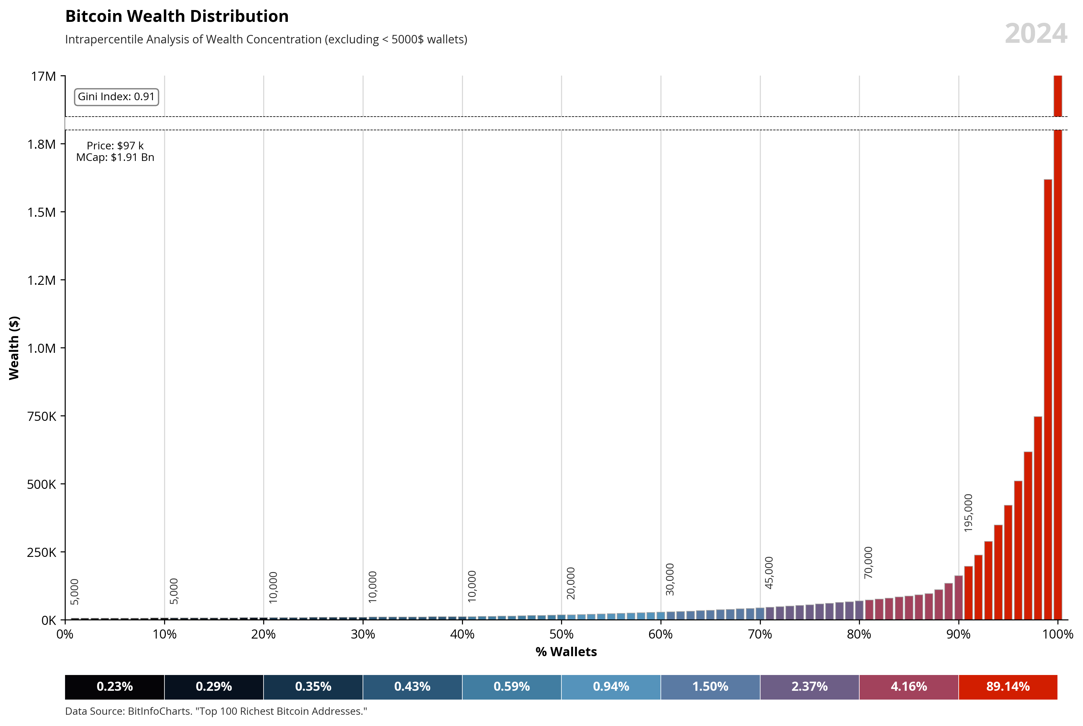
Critiques the concentration of Bitcoin wealth, exploring how its distribution aligns with ideals of anarcho-capitalism, where economic power is concentrated among a few, often bypassing traditional systems.
Published
Mar 4, 2025
Keywords
Bitcoin
Summary
A plot that shows the distribution wealth of Bitcoin among the wallets with a balance greater than $5,000 USD.
Code
# Libraries# ===================================================import pandas as pdimport numpy as npfrom bs4 import BeautifulSoupimport requestsfrom io import StringIOimport matplotlib.pyplot as pltfrom matplotlib.ticker import FuncFormatterimport matplotlib.patches as patches# Bitcoin Price# ===================================================url ="https://min-api.cryptocompare.com/data/price?fsym=BTC&tsyms=USD"response = requests.get(url)data = response.json()btcprice = data.get("USD")# Bitcoin Supply# ===================================================def get_btc_supply(): response = requests.get("https://blockchain.info/q/totalbc") satoshi =int(response.text) btcsupply = satoshi /100000000return btcsupplybtcsupply = get_btc_supply()# Data Extraction# ===================================================url ="https://bitinfocharts.com/top-100-richest-bitcoin-addresses.html"soup = BeautifulSoup(requests.get(url).text, "html.parser")table = soup.find("table", {"class": "table table-condensed bb"})df = pd.read_html(StringIO(str(table)))[0]# Data Transformation# ===================================================# Select columnsdf = df[['Balance, BTC', 'Addresses', 'BTC']]# Rename columns and add averagedf.rename(columns={'Addresses': 'rows', 'BTC': 'btc'}, inplace=True)# Extract start and end rangedf['start'] = df['Balance, BTC'].str.extract(r'[\[\(](\d[\d,\.]*)')df['end'] = df['Balance, BTC'].str.extract(r'-\s([\d,\.]+)\)')df['btc'] = df['btc'].str.extract('([0-9.]+)')# Convert to valuesdf['rows'] = df['rows'].replace({',': ''}, regex=True).astype(int)df['start'] = df['start'].replace({',': ''}, regex=True).astype(float)df['end'] = df['end'].replace({',': ''}, regex=True).astype(float)df['btc'] = df['btc'].replace({',': ''}, regex=True).astype(float)# Add average pricedf['average'] = df['btc'] / df['rows']# Select columnsdf = df[['rows', 'start', 'end', 'btc', 'average']]# Change first and last valuedf.loc[df.index[0], 'start'] =0.000001df.loc[df.index[-1], 'end'] =250000# Create a listresult = []# Iterate over each row for index, row in df.iterrows(): n =int(row['rows']) start = row['start'] end = row['end'] average = row['average']# Generate a distribution valores = np.logspace(np.log(start) / np.log(12), np.log(end) / np.log(12), n)# Calcular el factor de escala para ajustar el promedio current_average = np.mean(valores) scale_factor = average / current_average adjusted_values = valores * scale_factor# Add values to result list result.extend(valores)# Crear a dataframe with all valuesdf = pd.DataFrame(result, columns=['btc'])# Calculate marketcapmarketcap = btcsupply * btcprice# USD Value, Filter >5000 and countdf['usd'] = df['btc'] * btcpricedf = df[df['usd'] >5000]df['count'] =1# Grouping by 100 percentilesdf['percentile'] = pd.qcut(df['btc'], 100, labels=False) +1# Grouping by 10 percentilesdf['percentile2'] = pd.cut( df['percentile'], bins=range(1, 111, 10), right=False, labels=[i +9for i inrange(1, 101, 10)]).astype(int)# Calculate GINI Indexdef gini(x): x = np.array(x) x = np.sort(x) n =len(x) gini_index = (2* np.sum(np.arange(1, n +1) * x) - (n +1) * np.sum(x)) / (n * np.sum(x))return gini_indexgini_value = gini(df['usd'])# Summarizing data df = df.groupby(['percentile', 'percentile2'])[['usd', 'btc', 'count']].sum().reset_index()# Average pricedf['average_usd'] = df['usd'] / df['count']df['percentage'] = df['usd'] / df['usd'].sum()# Select columnsdf = df[['percentile', 'percentile2', 'usd', 'count', 'average_usd', 'percentage']]# Define palettecolor_palette = {10: "#050407",20: "#07111e",30: "#15334b",40: "#2b5778",50: "#417da1",60: "#5593bb",70: "#5a7aa3",80: "#6d5e86",90: "#a2425c",100: "#D21E00"}# Map palette colordf['color'] = df['percentile2'].map(color_palette)# Percentiles dataframe 2df2 = df.copy()df2 = df2.groupby(['percentile2', 'color'], as_index=False)[['usd', 'count']].sum()df2['average_usd'] = df2['usd'] / df2['count']df2['percentage'] = df2['usd'] / (df2['usd']).sum()df2['count'] =10print(df)# Data Visualization# ===================================================# Font Styleplt.rcParams.update({'font.family': 'sans-serif', 'font.sans-serif': ['Open Sans'], 'font.size': 10})# Create the figure and suplotsfig, (ax1, ax2) = plt.subplots(2, 1, figsize=(12, 8), gridspec_kw={'height_ratios': [10, 0.5]})# First Plot# ==================# Plot Barsbars = ax1.bar(df['percentile'], df['average_usd'], color=df['color'], edgecolor='darkgrey', linewidth=0.5, zorder=2)# Title and labelsax1.text(0, 1.1, 'Bitcoin Wealth Distribution', fontsize=13, fontweight='bold', ha='left', transform=ax1.transAxes)ax1.text(0, 1.06, 'Intrapercentile Analysis of Wealth Concentration (excluding < 5000$ wallets)', fontsize=9, color='#262626', ha='left', transform=ax1.transAxes)ax1.set_xlabel('% Wallets', fontsize=10, weight='bold')ax1.set_ylabel('Wealth ($)', fontsize=10, weight='bold')# Configurationax1.grid(axis='x', linestyle='-', alpha=0.5, zorder=1)ax1.set_xlim(0, 101)ax1.set_ylim(0, 2000000)ax1.set_xticks(np.arange(0, 101, step=10))ax1.set_yticks(np.arange(0, 2000001, step=250000))ax1.tick_params(axis='x', labelsize=10)ax1.tick_params(axis='y', labelsize=10)ax1.spines['top'].set_visible(False)ax1.spines['right'].set_visible(False)# Function to format Y axisdef format_func(value, tick_number):if value >=1e6:return'{:,.1f}M'.format(value /1e6)else:return'{:,.0f}K'.format(value /1e3)# Formatting x and y axisax1.xaxis.set_major_formatter(FuncFormatter(lambda x, _: f'{x:.0f}%'))ax1.yaxis.set_major_formatter(FuncFormatter(format_func))# Lines and area to separate outliersax1.axhline(y=1850000, color='black', linestyle='--', linewidth=0.5, zorder=4)ax1.axhline(y=1800000, color='black', linestyle='--', linewidth=0.5, zorder=4)ax1.add_patch(patches.Rectangle((0, 1800000), 105, 50000, linewidth=0, edgecolor='none', facecolor='white', zorder=3))# Y Axis modify the outlier valuelabels = [item.get_text() for item in ax1.get_yticklabels()]labels[-1] ='17M'ax1.set_yticklabels(labels)# Show labels each 10 percentilefor i, (bar, value) inenumerate(zip(bars, df['average_usd'])): value_rounded =round(value /5000) *5000if i %10==0: ax1.text(bar.get_x() + bar.get_width() /2, abs(bar.get_height()) *1.4+50000,f'{value_rounded:,.0f}', ha='center', va='bottom', fontsize=8.5, color='#2c2c2c', rotation=90)# Show GINI Indexax1.text(0.09, 0.97, f"Gini Index: {gini_value:.2f}", transform=ax1.transAxes, fontsize=8.5, color='black', ha='right', va='top', bbox=dict(boxstyle="round,pad=0.3", edgecolor='gray', facecolor='white'))# Show MarketCapax1.text(0.05, 0.88, f"Price: ${btcprice /1e3:.0f} k\nMCap: ${marketcap /1e12:.2f} Bn", transform=ax1.transAxes, fontsize=8.5, color='black', ha='center', va='top')# Second Plot# ==================# Plot Barsax2.barh([0] *len(df2), df2['count'], left=df2['percentile2'] - df2['count'], color=df2['color'])# Configurationax2.grid(axis='x', linestyle='-', color='white', alpha=1, linewidth=0.5)ax2.tick_params(axis='x', which='both', bottom=False, top=False, labelbottom=False)ax2.tick_params(axis='y', which='both', left=False, right=False, labelleft=False)ax2.spines['top'].set_visible(False)ax2.spines['right'].set_visible(False)ax2.spines['left'].set_visible(False)ax2.spines['bottom'].set_visible(False)x_ticks = np.linspace(df2['percentile2'].min(), df2['percentile2'].max(), 10)ax2.set_xticks(x_ticks)ax2.set_xlim(0, 101)# Add label valuesfor i, row in df2.iterrows(): plt.text(row['percentile2'] - row['count'] + row['count'] /2, 0, f'{row["percentage"] *100:.2f}%', ha='center', va='center', color='white', fontweight='bold')# Add Year labelformatted_date =2024ax1.text(1, 1.1, f'{formatted_date}', transform=ax1.transAxes, fontsize=22, ha='right', va='top', fontweight='bold', color='#D3D3D3')# Add Data Sourceax2.text(0, -0.5, 'Data Source: BitInfoCharts. "Top 100 Richest Bitcoin Addresses."', transform=ax2.transAxes, fontsize=8, color='#2c2c2c')# Adjust layoutplt.tight_layout()# Save it...plt.savefig("C:/Users/guill/Downloads/FIG_BITINFO_Bitcoin_Wealth_Distribution.png", dpi=300, bbox_inches='tight') # Plot it!plt.show()