Alquiler de vivienda en Catalunya: Distribución de precios

Los gráficos muestran la distribución de precios en los anuncios de alquiler ofertados en la plataforma de Idealista en Enero de 2025

Keywords

Alquiler

Summary

Representación de los precios de aquiler por comarca.

# Libraries
# ===================================
library(readr)
library(dplyr)
library(ggplot2)
library(ggdist)
library(ggtext)
library(scales)
library(grid)

# Extract Data
# ===================================
# URL GitHub
url <- "https://raw.githubusercontent.com/guillemmaya92/Python/main/Data/Catalunya_CP.csv"

# Read CSV
df <- read_delim(url, delim = ";", locale = locale(encoding = "latin1"))

# Select relevant columns and filter data
df <- df %>%
  select(province, region, price) %>%
  filter(region %in% c("Barcelonès") & price < 3000) %>%
  filter(!is.na(price))

# Transform Data
# ===================================
# Define values
min_price <- 0
cheaper_price <- 800
median_price <- median(df$price, na.rm = TRUE)
max_price <- 3000
total_announcements <- nrow(df)

# Calculate extra label values
mid1 <- (cheaper_price + min_price) / 2
announcements1 <- nrow(df %>% filter(price > min_price & price <= cheaper_price))
mid2 <- (median_price + cheaper_price) / 2
announcements2 <- nrow(df %>% filter(price > cheaper_price & price <= median_price))
mid3 <- (max_price + median_price) / 2
announcements3 <- nrow(df %>% filter(price > median_price & price <= max_price))

# Add color column
df <- df %>%
  mutate(color = case_when(
    price < cheaper_price ~ "#ffc939",
    price < median_price ~ "#a8c2d2",
    TRUE ~ "#477794"
  ))

# Show data
print(head(df))

# Plot Data
# ===================================
gg <- df %>%
  # Create ggplot
  ggplot(aes(x = price, fill = after_stat(case_when(
    x <= cheaper_price ~ "cheaper",
    x <= median_price ~ "median",
    TRUE ~ "expensive"
  )))) +
  # Define type of plot
  geom_dots(
    smooth = smooth_bounded(adjust = 0.6), 
    side = "both", 
    color = NA,
    dotsize = 0.8,
    stackratio = 1.3
  ) +
  # Configure XY Axis
  scale_x_continuous(
    limits = c(min_price, max_price),
    breaks = seq(min_price, max_price, by = 200),
    labels = scales::comma_format()
  ) +
  scale_y_continuous(breaks = NULL) +
  # Configure Titles and Captions
  labs(
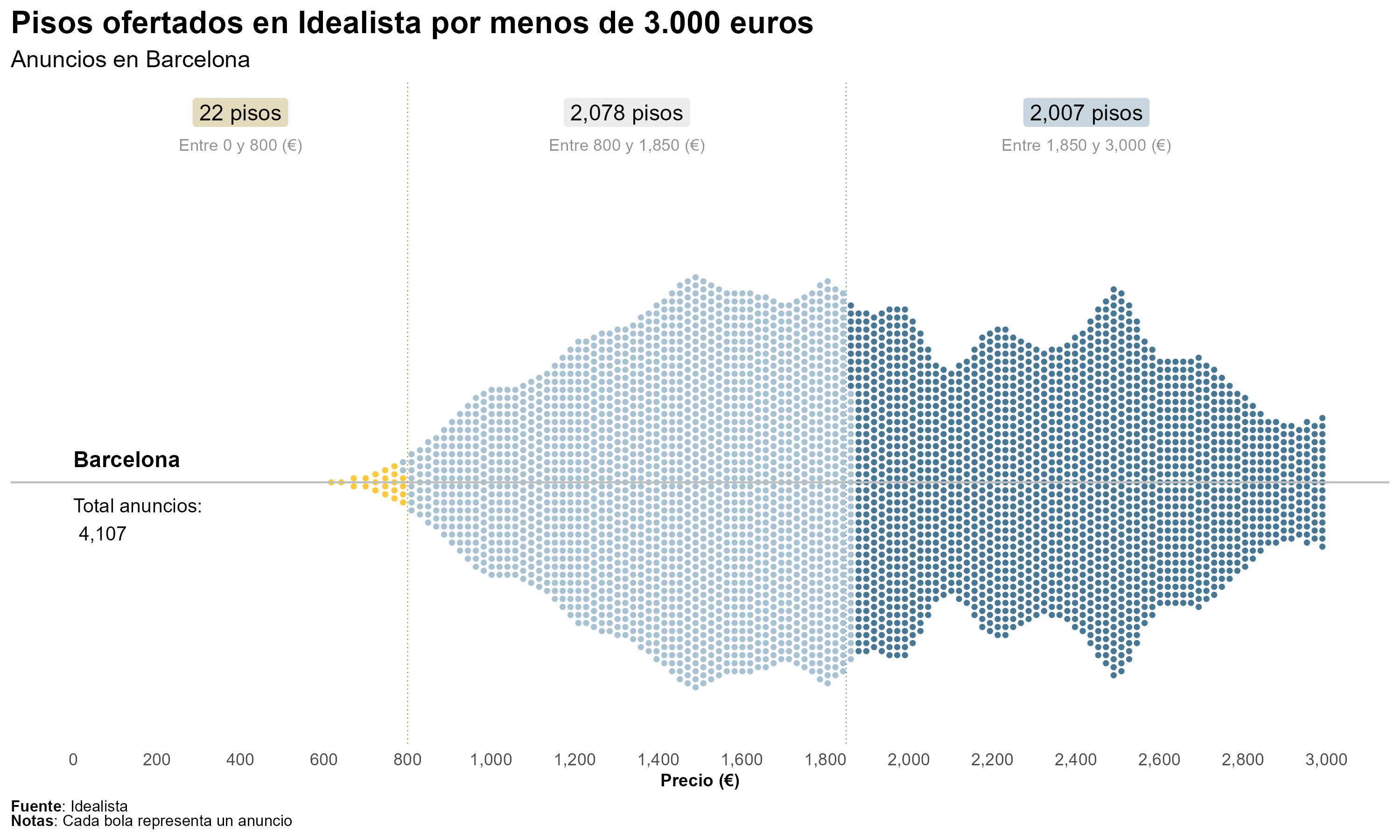
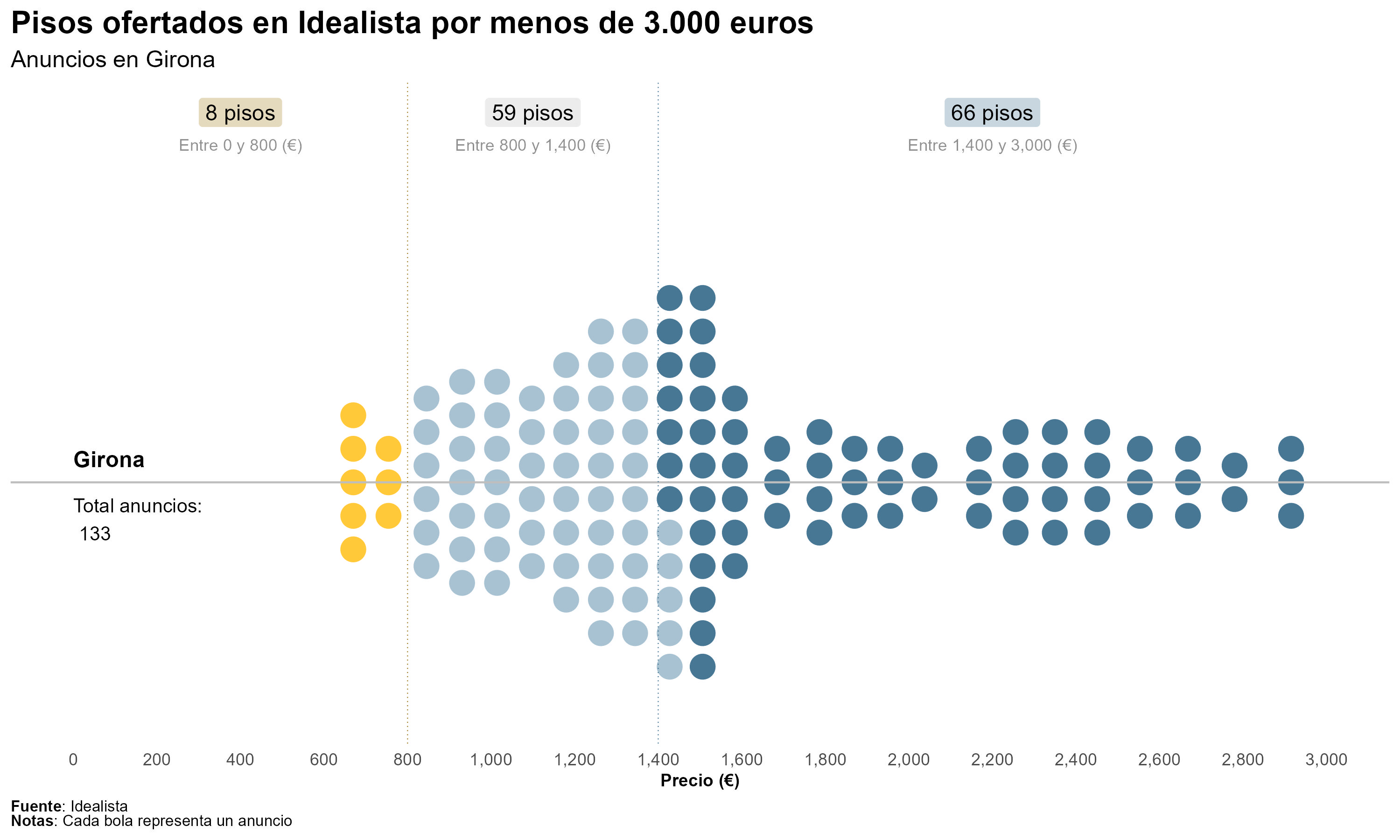
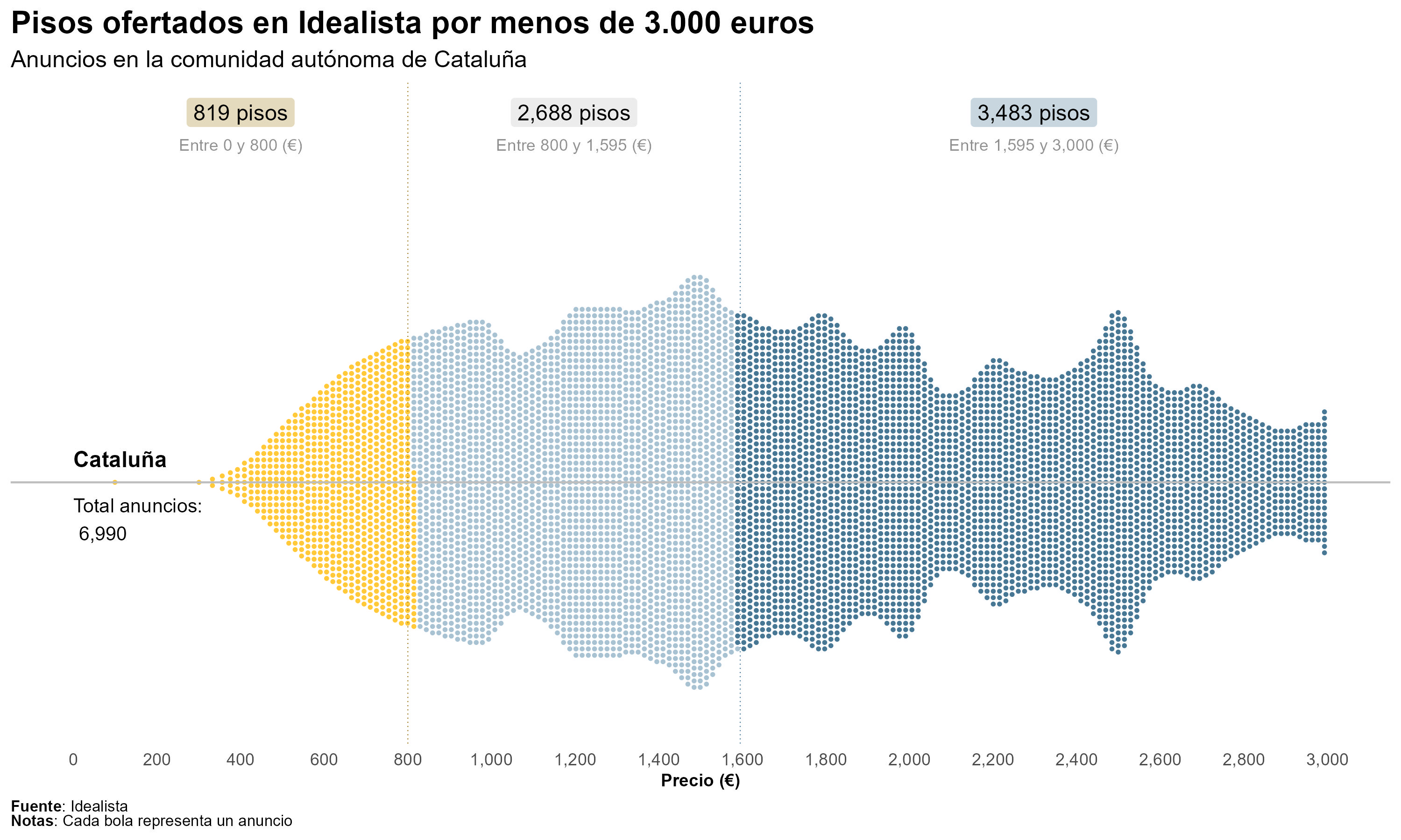
    title = 'Pisos ofertados en Idealista por menos de 3.000 euros',
    subtitle = "Anuncios en la comarca del Barcelonés",
    x = "Precio (€)",
    caption = paste0(
      "**Fuente**: Idealista<br>
      **Notas**: Cada bola representa un anuncio"
    )
  ) +
  # Configure elements theme
  theme_minimal() +
  theme(
    plot.title = element_text(size = 16, face = "bold"),
    plot.subtitle = element_text(size = 12, face = "plain"),
    axis.title.x = element_text(size = 9, face = "bold"),
    axis.title.y = element_blank(),
    panel.grid.major.x = element_blank(),
    panel.grid.minor.x = element_blank(),
    panel.grid.major.y = element_blank(),
    panel.grid.minor.y = element_blank(),
    legend.position = "none",
    plot.caption = element_markdown(size = 8, hjust = 0)
  ) +
 # Configure fill colors after_stats
  scale_fill_manual(values = c(
    "cheaper" = "#ffc939",
    "median" = "#a8c2d2",
    "expensive" = "#477794"
  )) +
  # Plot Vertical And Horizontal lines
  geom_hline(yintercept = 0, linetype = "solid", color = "grey", size = 0.5) +
  geom_vline(xintercept = cheaper_price, color = "#9c7a1f", linetype = "dotted", size = 0.25) +
  geom_vline(xintercept = median_price, color = "#477794", linetype = "dotted", size = 0.25) +
  # Annotate: City and adds 
  annotate("text", 
           x = 0, 
           y = 0.05, 
           label = "Barcelonés", 
           size = 4, 
           color = "black", 
           fontface = "bold", 
           hjust = 0) +
  annotate("text", 
           x = 0, 
           y = -0.08, 
           label = paste("Total anuncios:\n", comma(total_announcements)), 
           size = 3.5, 
           color = "black", 
           fontface = "plain", 
           hjust = 0) +
  # Annotate G1: Cheap adds
  annotate(geom = "label", 
           x = mid1, 
           y = 0.8, 
           label = paste(comma(announcements1), "pisos"), 
           size = 4, 
           color = "black", 
           fontface = "plain",
           fill = "#a68221",
           alpha = 0.3,
           label.size = 0) +
  annotate(geom = "text", 
           x = mid1, 
           y = 0.73, 
           label = paste("Entre", comma(min_price), "y", comma(cheaper_price), "(€)"), 
           size = 3, 
           color = "#909090") +
  # Annotate G2: Median adds
  annotate(geom = "label", 
           x = mid2, 
           y = 0.8, 
           label = paste(comma(announcements2), "pisos"), 
           size = 4, 
           color = "black", 
           fontface = "plain",
           fill = "grey",
           alpha = 0.3,
           label.size = 0) +
  annotate(geom = "text", 
           x = mid2, 
           y = 0.73, 
           label = paste("Entre", comma(cheaper_price), "y", comma(median_price), "(€)"), 
           size = 3, 
           color = "#909090") +
  # Annotate G3: Expensive adds
  annotate(geom = "label", 
           x = mid3, 
           y = 0.8, 
           label = paste(comma(announcements3), "pisos"), 
           size = 4, 
           color = "black", 
           fontface = "plain",
           fill = "#477794",
           alpha = 0.3,
           label.size = 0) +
  annotate(geom = "text", 
           x = mid3, 
           y = 0.73, 
           label = paste("Entre", comma(median_price), "y", comma(max_price), "(€)"), 
           size = 3, 
           color = "#909090") +
  # Extra Annotation: @Author
  annotation_custom(
    grob = textGrob("@damnedliestats", gp = gpar(fontsize = 8, col = "black")), 
    xmin = 2600, xmax = 3000, ymin = -0.73, ymax = -0.73
  ) +
  # Allow extra elements
  coord_cartesian(clip = "off")

# Saving Plot
ggsave("C:/Users/guill/Downloads/Barcelonés.jpeg", 
       plot = gg, dpi = 300, width = 10, height = 6)