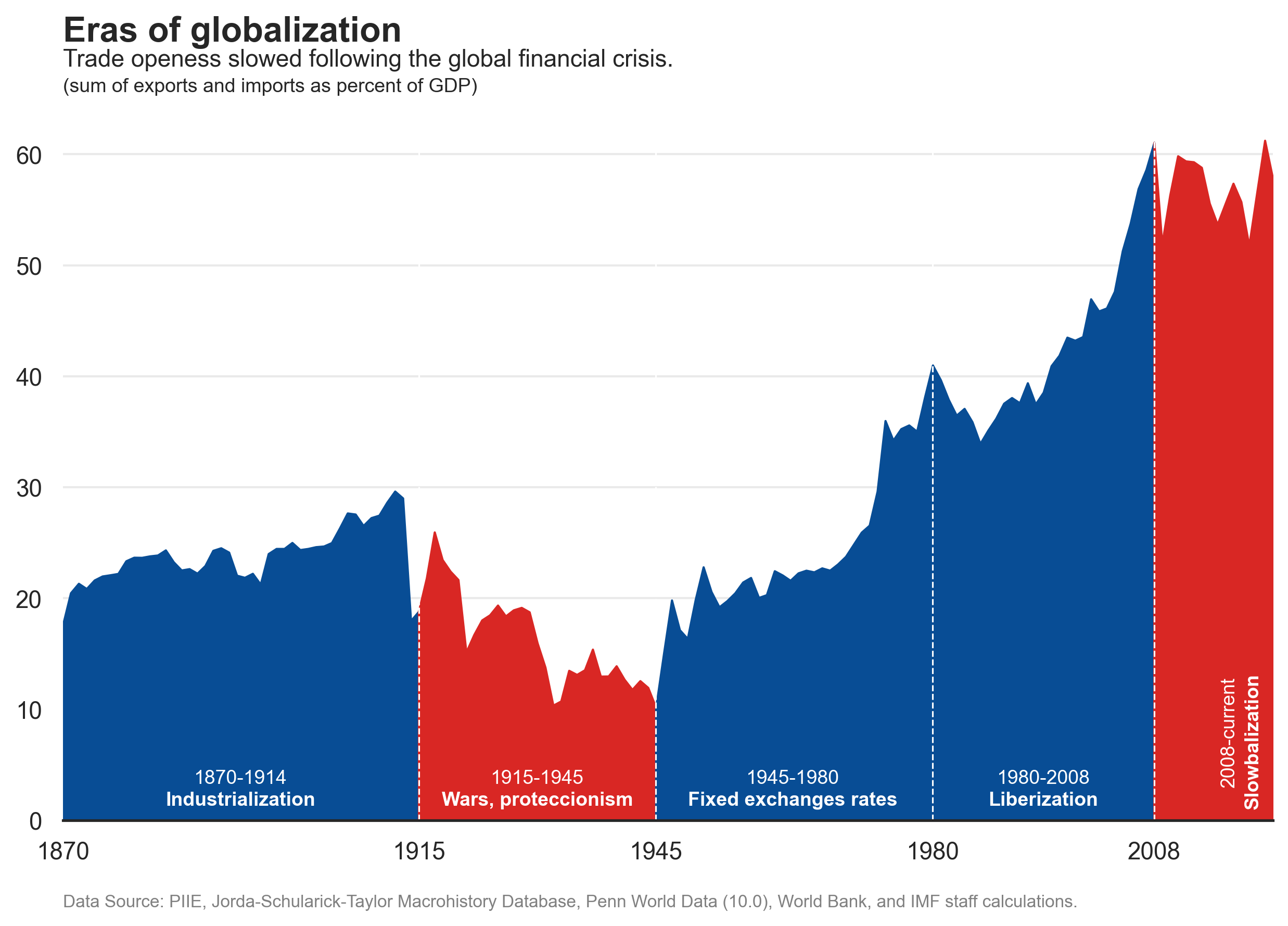
The pace of globalization slowed in the decade and a half since the global financial crisis, resulting in an era often referred to as “slowbalization
Published
Oct 9, 2025
Keywords
wealth-income
Summary
The chart illustrates the level of openness in global trade since the onset of globalization, with each period marked by unique economic conditions and distinct international relations.
Code
# Libraries# ============================================import pandas as pdimport numpy as npimport requestsimport wbgapi as wbimport matplotlib.pyplot as pltimport seaborn as sns# Extraction Data OURWORLDINDATA# ============================================# Get datadfo = pd.read_csv("https://ourworldindata.org/grapher/globalization-over-5-centuries.csv?v=1&csvType=full&useColumnShortNames=true", storage_options = {'User-Agent': 'Our World In Data data fetch/1.0'})dfo = dfo[dfo['Code'] =='OWID_WRL']# Rename columnsdfo = dfo.rename(columns={'Year': 'year',' World trade based on Maddison (% of GDP) (Klasing and Milionis (2014)) ': 'trade_klasing','World trade based on own estimates (% of GDP) (Klasing and Milionis (2014)) ': 'trade_klasing_madisson','ne_trd_gnfs_zs': 'trade_penn','trade_openness': 'trade_openness_index'})# Trade priority datadfo = dfo[['year', 'trade_klasing', 'trade_klasing_madisson', 'trade_penn', 'trade_openness_index']]dfo['trade'] = np.where(dfo['trade_openness_index'].notnull(), dfo['trade_openness_index'], np.where(dfo['trade_penn'].notnull(), dfo['trade_penn'], np.where(dfo['trade_klasing_madisson'].notnull(), dfo['trade_klasing_madisson'], dfo['trade_klasing'])))# Prepare dfodfo = dfo[['year', 'trade']]dfo = dfo[dfo['trade'].notnull()]dfo = dfo.sort_values(by='year').reset_index(drop=True)# Extraction Data COUNTRIES# =====================================================================# Extract JSON and bring data to a dataframeurl ='https://raw.githubusercontent.com/guillemmaya92/world_map/main/Dim_Country.json'response = requests.get(url)data = response.json()dfc = pd.DataFrame(data)dfc = pd.DataFrame.from_dict(data, orient='index').reset_index()df_countries = dfc.rename(columns={'index': 'ISO3'})# Extraction Data WORLDBANK# ========================================================# To use the built-in plotting methodindicator = ['NY.GDP.MKTP.CD', 'NE.EXP.GNFS.CD', 'NE.IMP.GNFS.CD']countries = df_countries['ISO3'].tolist()data_range =range(1970, 2024)data = wb.data.DataFrame(indicator, 'WLD', data_range, numericTimeKeys=True, labels=False, columns='series').reset_index()dfw = data.rename(columns={'time': 'year','economy': 'iso','NY.GDP.MKTP.CD': 'gdp','NE.EXP.GNFS.CD': 'exports','NE.IMP.GNFS.CD': 'imports'})dfw['comerce'] = dfw['imports'] + dfw['exports']dfw = dfw[['year', 'gdp', 'comerce']].groupby('year', as_index=False).sum()dfw['trade'] = dfw['comerce'] / dfw['gdp'] *100dfw = dfw[['year', 'trade']]# Unify DF# ========================================================# Filter dataframesdfo = dfo[dfo['year'] <1970]dfw = dfw[dfw['year'] >1970]# Filter dataframesdf = pd.concat([dfo, dfw], ignore_index=True)# Divide dataframesdf_1870_1914 = df[(df['year'] >=1870) & (df['year'] <=1915)]df_1915_1945 = df[(df['year'] >=1915) & (df['year'] <=1945)]df_1945_1980 = df[(df['year'] >=1945) & (df['year'] <=1980)]df_1980_2008 = df[(df['year'] >=1980) & (df['year'] <=2008)]df_2008_2023 = df[(df['year'] >=2008) & (df['year'] <=2023)]print(df)# Visualization Data# ============================================# Font and styleplt.rcParams.update({'font.family': 'sans-serif', 'font.sans-serif': ['Open Sans'], 'font.size': 10})sns.set(style="white", palette="muted")# Create a figureax = plt.figure(figsize=(10, 6))# Stackplot for each dataframeplt.stackplot(df_1870_1914['year'], df_1870_1914['trade'], color='#084d95', alpha=1)plt.stackplot(df_1915_1945['year'], df_1915_1945['trade'], color='#d92724', alpha=1)plt.stackplot(df_1945_1980['year'], df_1945_1980['trade'], color='#084d95', alpha=1)plt.stackplot(df_1980_2008['year'], df_1980_2008['trade'], color='#084d95', alpha=1)plt.stackplot(df_2008_2023['year'], df_2008_2023['trade'], color='#d92724', alpha=1)# Add vertical linesplt.axvline(x=1915, color='white', linestyle='--', linewidth=0.75)plt.axvline(x=1945, color='white', linestyle='--', linewidth=0.75)plt.axvline(x=1980, color='white', linestyle='--', linewidth=0.75)plt.axvline(x=2008, color='white', linestyle='--', linewidth=0.75)# Add title and labelsplt.text(0, 1.08, f'Eras of globalization', fontsize=16, fontweight='bold', ha='left', transform=plt.gca().transAxes)plt.text(0, 1.045, 'Trade openess slowed following the global financial crisis.', fontsize=11, color='#262626', ha='left', transform=plt.gca().transAxes)plt.text(0, 1.01, '(sum of exports and imports as percent of GDP)', fontsize=9, fontweight='light', color='#262626', ha='left', transform=plt.gca().transAxes)plt.xlim(1871, 2023)plt.ylim(0, 65)plt.xticks([1870, 1915, 1945, 1980, 2008])plt.gca().yaxis.grid(True, linestyle='-', alpha=0.4)# Delete spinesfor spine in ["top", "left", "right"]: plt.gca().spines[spine].set_visible(False)# Industrializationplt.text( x=df_1870_1914['year'].mean(), y=3, s="1870-1914", fontsize=9, color='white', ha='center', va='bottom')plt.text( x=df_1870_1914['year'].mean(), y=1, s="Industrialization", fontsize=9, fontweight='bold', color='white', ha='center', va='bottom')# Wars and proteccionismplt.text( x=df_1915_1945['year'].mean(), y=3, s="1915-1945", fontsize=9, color='white', ha='center', va='bottom')plt.text( x=df_1915_1945['year'].mean(), y=1, s="Wars, proteccionism", fontsize=9, fontweight='bold', color='white', ha='center', va='bottom')# Fixed exchanges ratesplt.text( x=df_1945_1980['year'].mean(), y=3, s="1945-1980", fontsize=9, color='white', ha='center', va='bottom')plt.text( x=df_1945_1980['year'].mean(), y=1, s="Fixed exchanges rates", fontsize=9, fontweight='bold', color='white', ha='center', va='bottom')# Liberizationplt.text( x=df_1980_2008['year'].mean(), y=3, s="1980-2008", fontsize=9, color='white', ha='center', va='bottom')plt.text( x=df_1980_2008['year'].mean(), y=1, s="Liberization", fontsize=9, fontweight='bold', color='white', ha='center', va='bottom')# Slowbalizationplt.text( x=df_2008_2023['year'].mean() +2, y=3, s="2008-current", fontsize=9, color='white', ha='center', va='bottom', rotation=90)plt.text( x=df_2008_2023['year'].mean() +5, y=1, s="Slowbalization", fontsize=9, fontweight='bold', color='white', ha='center', va='bottom', rotation=90)# Add Data Sourceplt.text(0, -0.12, 'Data Source: PIIE, Jorda-Schularick-Taylor Macrohistory Database, Penn World Data (10.0), World Bank, and IMF staff calculations.', transform=plt.gca().transAxes, fontsize=8, color='gray')# Show plot!plt.show()