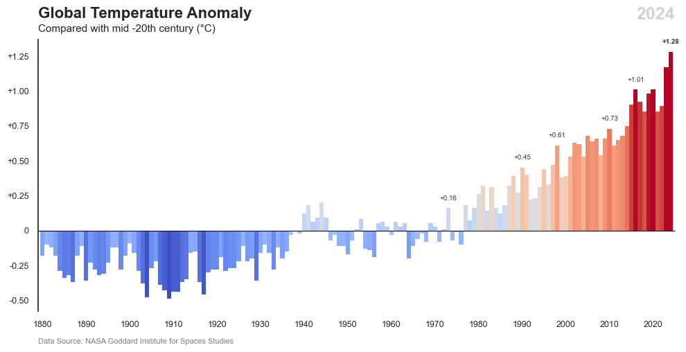
Revealing climate change through deviations in Earth’s surface temperature from the historical average.
Published
Nov 3, 2025
Keywords
temperature
Summary
Global temperature anomalies indicate how Earth’s surface temperature deviates from a historical average, providing crucial insights into climate change. Persistent positive anomalies signal a warming trend driven by greenhouse gas emissions, while negative anomalies are less frequent in recent decades. By tracking these variations, scientists can assess long-term climate patterns, identify extreme weather risks, and evaluate the impact of human activities on global temperatures.
Code
# Libraries# =========================================import pandas as pdimport numpy as npimport matplotlib.pyplot as pltimport seaborn as snsimport matplotlib.ticker as tickerimport os# Data Extraction (temperature)# =========================================# URL NASA GISS global temperatureurl ="https://data.giss.nasa.gov/gistemp/tabledata_v4/GLB.Ts+dSST.csv"dft = pd.read_csv(url, skiprows=1)# Data Extraction (co2)# =========================================# URL del archivo CSVurl ="https://zenodo.org/records/13981696/files/GCB2024v17_MtCO2_flat.csv?download=1"dfc = pd.read_csv(url)# Data Manipulation (temperature)# =========================================# Select columnsdft = dft[["Year", "Jan", "Feb", "Mar", "Apr", "May", "Jun", "Jul", "Aug", "Sep", "Oct", "Nov", "Dec", "J-D"]]# Rename columnsdft.columns = dft.columns.str.lower()dft = dft.rename(columns=lambda x: x.lower())# Unpivot columnsdft = dft.melt(id_vars=["year"], var_name="month", value_name="value")dft = dft[dft["month"] =="j-d"]# Data Manipulation (co2)# =========================================# Transform Datadfc = dfc[dfc['ISO 3166-1 alpha-3'] =='WLD']dfc.rename(columns={'Year': 'year', 'ISO 3166-1 alpha-3': 'iso', 'Total': 'co2'}, inplace=True)dfc = dfc[['year', 'iso', 'co2']]# Merge dataframes# =========================================df = dft.merge(dfc, on='year', how='left')df['value'] = pd.to_numeric(df['value'], errors='coerce')df = df[df['value'].notna()]print(df)# Data Visualization# =========================================# Font and styleplt.rcParams.update({'font.family': 'sans-serif', 'font.sans-serif': ['Open Sans'], 'font.size': 9})sns.set(style="white", palette="muted")# Define a color mapcmap = plt.get_cmap('coolwarm')norm = plt.Normalize(-0.5, 1)# Create figure and plotfig, ax1 = plt.subplots(figsize=(10, 5))ax2 = ax1.twinx()bars =ax1.bar(df['year'], df['value'], color=cmap(norm(df['value'])), width=1, edgecolor='none')line = ax2.plot(df['year'], df['co2'], label='CO2', color='#262626', linestyle=':', linewidth=1)# Add title and labelsax1.text(0, 1.12, f'Global Temperature Anomaly', fontsize=16, fontweight='bold', ha='left', transform=ax1.transAxes)ax1.text(0, 1.07, 'Compared with mid -20th century (°C)', fontsize=11, color='#262626', ha='left', transform=ax1.transAxes)ax1.text(0, 1.02, r'(In contrast with CO$_2$ emissions)', fontsize=9, fontweight='light', color='#262626', ha='left', transform=ax1.transAxes)ax1.set_xlim(1877, 2027)ax1.axhline(y=0, color='black', linestyle='-', linewidth=0.75)yticks = [-0.5, -0.25, 0, 0.25, 0.5, 0.75, 1, 1.25]ytick_labels = [f'{y:+.2f}'if y !=0else'0'for y in yticks]ax1.set_yticks(yticks, ytick_labels)ax1.set_yticklabels(ytick_labels, fontsize=9)ax1.set_xticks([1880, 1890, 1900, 1910, 1920, 1930, 1940, 1950, 1960, 1970, 1980, 1990, 2000, 2010, 2020])ax1.tick_params(axis='x', labelsize=9)ax1.yaxis.set_ticks_position('none')ax1.grid(axis='y', linestyle='-', color='#262626', linewidth=0.1, alpha=0.6)ax2.set_ylim(0, 40000)ymin, ymax = ax2.get_ylim()yticks = np.linspace(ymin, ymax, 8)ax2.set_yticks(yticks)yticks_rounded = np.round(yticks /5000) *5000yticks_k = [f"{int(tick /1000)}Mt"for tick in yticks_rounded]ax2.set_yticklabels(yticks_k)ax2.tick_params(axis='y', labelsize=9)ax2.yaxis.set_ticks_position('none')# Add column labelsfor i, year inenumerate(df['year']):if year in [1973, 1990, 1998, 2010, 2016, 2024]:# Check positive and negative values symbol ="+"if df['value'].iloc[i] >=0else"-" value_text =f"{symbol}{abs(df['value'].iloc[i]):,.2f}"# Recent value bold fontweight ='bold'if year == df['year'].max() else'normal'# Set the offset based on the year offset =0.11if year in [1973, 1990] else0.05# Add label ax1.text(year, df['value'].iloc[i] + offset, value_text, ha='center', va='bottom', fontsize=7, color='#363636', fontweight=fontweight)# Remove spinesfor ax in [ax1, ax2]:for spine in ["top", "bottom"]: ax.spines[spine].set_visible(False)# Add Data Sourcespaces =' '*23ax1.text(0, -0.16, f'{spaces}NASA Goddard Institute for Space Studies\nThe Global Carbon Project\'s fossil CO2 emissions dataset', transform=ax1.transAxes, fontsize=8, color='gray', ha='left', family='sans-serif')# Add Data Source boldax1.text(0, -0.16, 'Data Source:\n ', transform=ax1.transAxes, fontsize=8, color='gray', ha='left', family='sans-serif', fontweight='bold')# Add Year labelformatted_date =2024ax1.text(1, 1.12, f'{formatted_date}', transform=ax1.transAxes, fontsize=18, ha='right', va='top', fontweight='bold', color='#D3D3D3')# Add Celsiusax1.text(-0.04, -0.08, '°C', transform=ax1.transAxes, fontsize=10, fontweight='bold', color='black')# Add CO2ax1.text(1.01, -0.08, r'CO$_2$', transform=ax1.transAxes, fontsize=10, fontweight='bold', color='black')# Adjust layoutplt.tight_layout()# Save it...download_folder = os.path.join(os.path.expanduser("~"), "Downloads")filename = os.path.join(download_folder, f"FIG_NASA_Temperature_Anomalies")plt.savefig(filename +".png", format='png', bbox_inches='tight')# Show the plot!plt.show()