Who absorbs the World’s surplus?

An analysis of global imbalance in the current account.

Keywords

exorbitant privilege

Summary

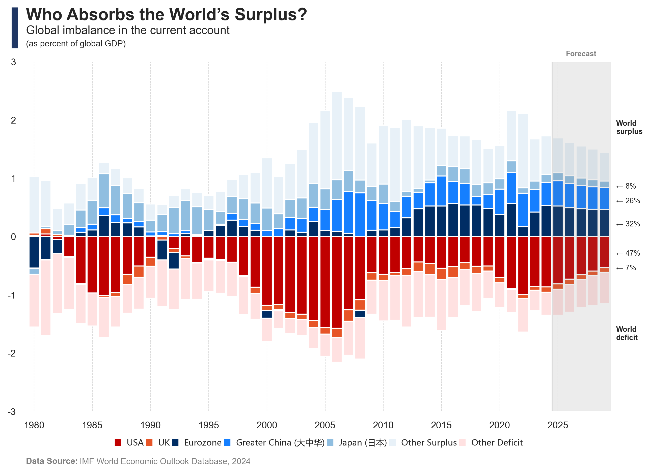
Global trade imbalances reveal structural asymmetries in the international financial system, with the United States playing a unique role due to the dominance of the U.S. dollar. While some economies accumulate surpluses, the U.S. consistently runs large trade deficits. This persistent imbalance is not simply a weakness but a reflection of the exorbitant privilege` of the dollar as the world’s primary reserve currency.

# Libraries
# =====================================================================
import os
import requests
import pandas as pd
import numpy as np
import seaborn as sns
import matplotlib.pyplot as plt
import matplotlib.patches as mpatches
import matplotlib.ticker as mticker
from matplotlib import font_manager

# Data Extraction (Countries)
# =====================================================================
# Extract JSON and bring data to a dataframe
url = 'https://raw.githubusercontent.com/guillemmaya92/world_map/main/Dim_Country.json'
response = requests.get(url)
data = response.json()
df = pd.DataFrame(data)
df = pd.DataFrame.from_dict(data, orient='index').reset_index()
df_countries = df.rename(columns={'index': 'ISO3'})

# Data Extraction (IMF)
# =====================================================================
#Parameter
parameters = ['BCA', 'NGDPD']

# Create an empty list
records = []

# Iterar sobre cada parámetro
for parameter in parameters:
    # Request URL
    url = f"https://www.imf.org/external/datamapper/api/v1/{parameter}"
    response = requests.get(url)
    data = response.json()
    values = data.get('values', {})

    # Iterate over each country and year
    for country, years in values.get(parameter, {}).items():
        for year, value in years.items():
            records.append({
                'Parameter': parameter,
                'ISO3': country,
                'Year': int(year),
                'Value': float(value)
            })
    
# Create dataframe
df_imf = pd.DataFrame(records)

# Data Manipulation
# =====================================================================
# Pivot Parameter to columns and filter nulls
df = df_imf.pivot(index=['ISO3', 'Year'], columns='Parameter', values='Value').reset_index()
df = df.dropna(subset=['BCA'], how='any')

# Merge queries
df = df.merge(df_countries, how='left', left_on='ISO3', right_on='ISO3')
df = df[['ISO3', 'Country', 'Year', 'BCA', 'NGDPD', 'Analytical', 'Region', 'Cod_Currency']]
df = df[df['Region'].notna()]

# Custom region
conditions = [
    df['ISO3'] == 'USA',
    df['ISO3'] == 'GBR',
    df['ISO3'].isin(['CHN', 'TWN', 'HKG', 'MAC']),
    df['ISO3'] == 'JPN',
    df['Cod_Currency'] == 'EUR',
    df['BCA'] >= 0,
    df['BCA'] < 0
]
result = ['USA', 'UK', 'Greater China', 'Japan', 'Eurozone', 'Other Surplus', 'Other Deficit']

df['Region'] = np.select(conditions, result)

# Groupping region and year
df = df.groupby(["Region", "Year"], as_index=False)[["BCA", "NGDPD"]].sum()

# Add total GDP
df['NGDPD'] = df.groupby('Year')['NGDPD'].transform('sum')
df['Ratio'] = df['BCA'] / df['NGDPD'] * 100

# Pivot Regions
df = df.pivot_table(index="Year", columns="Region", values="Ratio", aggfunc="sum")

# Reorder columns
df = df[["USA", "UK", "Eurozone", "Greater China", "Japan", "Other Surplus", "Other Deficit"]]

# Filter period
df = df.loc[df.index <= 2029]

# Values
usa_percent = df.loc[2029, 'USA'] / (df.loc[2029, 'Other Deficit'] + df.loc[2029, 'USA'] + df.loc[2029, 'UK'])
uk_percent = df.loc[2029, 'UK'] / (df.loc[2029, 'Other Deficit'] + df.loc[2029, 'USA'] + df.loc[2029, 'UK'])
eur_percent = df.loc[2029, 'Eurozone'] / (df.loc[2029, 'Other Surplus'] + df.loc[2029, 'Eurozone'] + df.loc[2029, 'Greater China'] + df.loc[2029, 'Japan'])
chn_percent = df.loc[2029, 'Greater China'] / (df.loc[2029, 'Other Surplus'] + df.loc[2029, 'Eurozone'] + df.loc[2029, 'Greater China'] + df.loc[2029, 'Japan'])
jpn_percent = df.loc[2029, 'Japan'] / (df.loc[2029, 'Other Surplus'] + df.loc[2029, 'Eurozone'] + df.loc[2029, 'Greater China'] + df.loc[2029, 'Japan'])

print(df)

# Data Visualization
# =====================================================================
# Font and style
plt.rcParams.update({'font.family': 'sans-serif', 'font.sans-serif': ['Franklin Gothic'], 'font.size': 9})
sns.set(style="white", palette="muted")

# Palette
palette = ["#C00000", "#E75527", "#002D64", "#157FFF", "#90bee0", "#E8F1F8", "#FFE1E1"]

# Create figure
fig, ax = plt.subplots(figsize=(10, 6))

# Crear figure and plot
ax = df.plot(kind="bar", stacked=True, width=0.9, color=palette, legend=False, ax=ax)

# Title
fig.add_artist(plt.Line2D([0.11, 0.11], [0.91, 1], linewidth=6, color='#203764', solid_capstyle='butt')) 
plt.text(0, 1.12, f'Who Absorbs the World’s Surplus?', fontsize=16, fontweight='bold', ha='left', transform=plt.gca().transAxes)
plt.text(0, 1.08, f'Global imbalance in the current account', fontsize=11, color='#262626', ha='left', transform=plt.gca().transAxes)
plt.text(0, 1.045, f'(as percent of global GDP)', fontsize=8, color='#262626', ha='left', transform=plt.gca().transAxes)

# Adjust ticks and grid
plt.ylim(-3, 3)
ax.set_xticks(range(0, 50, 5))  # Ajustar el rango con len(df)+1
ax.set_xticklabels(df.index[::len(df) // 10], fontsize=9, rotation=0)
ax.yaxis.set_major_formatter(mticker.FuncFormatter(lambda x, pos: f'{int(x):,}'.replace(",", ".")))
plt.gca().set_xlabel('')
plt.yticks(fontsize=9, color='#282828')
plt.grid(axis='x', linestyle='--', color='gray', linewidth=0.5, alpha=0.3)

# Custom legend values
handles = [
    mpatches.Patch(color=palette[0], label="USA", linewidth=2),
    mpatches.Patch(color=palette[1], label="UK", linewidth=2),
    mpatches.Patch(color=palette[2], label="Eurozone", linewidth=2),
    mpatches.Patch(color=palette[3], label="Greater China (大中华)", linewidth=2),
    mpatches.Patch(color=palette[4], label="Japan (日本)", linewidth=2),
    mpatches.Patch(color=palette[5], label="Other Surplus", linewidth=2),
    mpatches.Patch(color=palette[6], label="Other Deficit", linewidth=2)
]

# Legend
legend = plt.legend(
    handles=handles,
    loc='lower center', #center
    bbox_to_anchor=(0.5, -0.12),
    ncol=8,
    fontsize=8,
    frameon=False,
    handlelength=0.5,
    handleheight=0.5,
    borderpad=0.2,
    columnspacing=0.4
)
# legend.set_bbox_to_anchor((60, 0), transform=ax.transData)

# Change Font (accept chinese characters)
prop = font_manager.FontProperties(fname='C:\\Windows\\Fonts\\msyh.ttc')
for text in legend.get_texts():
    text.set_fontproperties(prop)
    text.set_fontsize(8)

# Add Data Source
plt.text(0, -0.15, 'Data Source:', 
    transform=plt.gca().transAxes, 
    fontsize=8,
    fontweight='bold',
    color='gray')
space = " " * 23
plt.text(0, -0.15, space + 'IMF World Economic Outlook Database, 2024', 
    transform=plt.gca().transAxes, 
    fontsize=8,
    color='gray')

# Add text
plt.text(50, -0.35, f"← {usa_percent:.0%}", fontsize=7, ha='left', va='bottom')
plt.text(50, -0.6, f"← {uk_percent:.0%}", fontsize=7, ha='left', va='bottom')
plt.text(50, 0.15, f"← {eur_percent:.0%}", fontsize=7, ha='left', va='bottom')
plt.text(50, 0.55, f"← {chn_percent:.0%}", fontsize=7, ha='left', va='bottom')
plt.text(50, 0.8, f"← {jpn_percent:.0%}", fontsize=7, ha='left', va='bottom')

plt.text(50, 2, f"World\nsurplus", fontsize=7, fontweight = 'bold', ha='left', va='top')
plt.text(50, -1.8, f"World\ndeficit", fontsize=7, fontweight = 'bold', ha='left', va='bottom')

# Forecast
plt.text(47, 3.1, f'Forecast', fontsize=7, fontweight='bold', color='gray', ha='center')
ax.axvspan(44.5, 49.5, color='gray', alpha=0.15, edgecolor='none')

# Remove spines
for spine in plt.gca().spines.values():
    spine.set_visible(False)

# Save it...
download_folder = os.path.join(os.path.expanduser("~"), "Downloads")
filename = os.path.join(download_folder, f"FIG_IMF_Global_Surplus.png")
plt.savefig(filename, dpi=300, bbox_inches='tight')

# Show :)
plt.show()

# Libraries
# ============================================
import pandas as pd
import numpy as np
import requests
import seaborn as sns
import matplotlib.pyplot as plt
import matplotlib.patches as mpatches
import matplotlib.ticker as ticker
import matplotlib.ticker as mticker
import os

# Data Countries
# ============================================
# URL countries
url = "https://www.census.gov/foreign-trade/schedules/c/country.txt"

# Read and clean the country data
dfc = (
    pd.read_csv(url, sep='|', header=None, skiprows=6, engine='python')
      .dropna(axis=1, how='all')
      .rename(columns={0: 'code', 1: 'name', 2: 'iso'})
)

# Select columns
dfc = dfc.astype(str).map(lambda x: x.strip())
dfc = dfc[['code', 'iso']]
dfc = dfc[dfc['code'].str.isdigit()]
dfc['code'] = dfc['code'].astype(int)

# Data Countries (Custom)
# =====================================================================
# Extract JSON and bring data to a dataframe
url = 'https://raw.githubusercontent.com/guillemmaya92/world_map/main/Dim_Country.json'
response = requests.get(url)
data = response.json()
dfgh = pd.DataFrame(data)
dfgh = pd.DataFrame.from_dict(data, orient='index').reset_index()
dfgh = dfgh.rename(columns={'index': 'iso3'})

# Data Extraction (XLSX)
# ============================================
# Read URL file
url = "https://www.census.gov/foreign-trade/balance/country.xlsx"
df = pd.read_excel(url)

# Remove and rename columns
df = df.drop(columns=['CTYNAME', 'IYR', 'EYR'], errors='ignore')
df = df.rename(columns={'CTY_CODE': 'code'})

# Traspose columns to rows
df = pd.melt(df, id_vars=['year', 'code'], var_name='month', value_name='value')

# Dictionary months
meses = {
    'JAN': 1, 'FEB': 2, 'MAR': 3, 'APR': 4, 'MAY': 5, 'JUN': 6,
    'JUL': 7, 'AUG': 8, 'SEP': 9, 'OCT': 10, 'NOV': 11, 'DEC': 12
}

# Define flow and mapping months 
df['flow'] = df['month'].str[0].map({'I': 'imports', 'E': 'exports'})
df['month'] = df['month'].str[-3:].map(meses)

# Create date column 
df['date'] = pd.to_datetime(dict(year=df['year'], month=df['month'], day=1))
df = df.drop(columns=['year', 'month'])

# Merge with country data
df['code'] = df['code'].astype(int)
df = df.merge(dfc, on='code', how='left')
df = df[['flow', 'iso', 'date', 'value']]
df = df[df['iso'].notna()] 

# Calculate balance
df['value'] = pd.to_numeric(df['value'], errors='coerce')
df = df.pivot_table(index=['iso', 'date'], columns='flow', values='value').reset_index()
df['balance'] = df['imports'].fillna(0) - df['exports'].fillna(0)

# Group by year
df['date'] = pd.to_datetime(df['date'])
df['year'] = df['date'].dt.year

# Group by countries
df = df.merge(dfgh, left_on='iso', right_on='ISO2', how='inner')
df = df[['iso', 'iso3', 'year', 'Cod_Currency', 'balance']]

# Data Extraction - IMF (1980-2030)
# =====================================================================
# Parametro
parameters = ['NGDPD']

# Create an empty list
records = []

# Iterar sobre cada parámetro
for parameter in parameters:
    # Request URL
    url = f"https://www.imf.org/external/datamapper/api/v1/{parameter}"
    response = requests.get(url)
    data = response.json()
    values = data.get('values', {})

    # Iterate over each country and year
    for country, years in values.get(parameter, {}).items():
        for year, value in years.items():
            records.append({
                'Parameter': parameter,
                'iso3': country,
                'year': int(year),
                'Value': float(value)
            })
    
# Create dataframe
df_imf = pd.DataFrame(records)

# Pivot Parameter to columns and filter nulls
df_imf = df_imf.pivot(index=['iso3', 'year'], columns='Parameter', values='Value').reset_index()
df_imf = df_imf[df_imf['iso3'] == 'USA']
df_imf = df_imf.drop(columns=['iso3'])

# Merge
df = df.merge(df_imf, on=['year'], how='inner')
df = df.rename(columns={'NGDPD': 'gdp'})

# Grouping 
conditions = [
    df['iso'] == 'CN',
    df['iso'] == 'TW',
    df['iso'] == 'VN',
    df['iso'] == 'JP',
    df['iso'] == 'KR',
    df['iso'] == 'TH',
    df['iso'] == 'IN',
]

choices = ['China', 'Taiwan', 'Vietnam', 'Japan', 'South Korea', 'Thailand', 'India']

df['group'] = np.select(conditions, choices, default='Rest of World')
df = df.groupby(['group', 'year'], as_index=False).agg({
    'balance': 'sum',
    'gdp': 'mean'
})
df = df[df['balance'] >= 0]

# Calculate ratio balance gdp
df['balance_gdp'] = df['balance'] / (df['gdp'] * 10)

# Data Visualization
# ============================================
# Font and style
plt.rcParams.update({'font.family': 'sans-serif', 'font.sans-serif': ['Franklin Gothic'], 'font.size': 9})
sns.set(style="white", palette="muted")

# Pivot and order columns
orden = ['China', 'Taiwan', 'Vietnam', 'Japan', 'South Korea', 'Thailand', 'India', 'Rest of World']
df_pivot = df.pivot(index='year', columns='group', values='balance_gdp')
df_pivot = df_pivot[[c for c in orden if c in df_pivot.columns]]

# Colors
palette = [
    '#D62728',  # China - rojo
    '#E84A1A',  # Taiwan - entre rojo y naranja
    '#FFA500',  # Vietnam - naranja
    '#FFD700',  # Japan - amarillo fuerte
    '#E6E655',  # South Korea - amarillo verdoso
    '#A9C94C',  # Thailand - verde amarillento
    "#809C2E",  # India - verde amarillento
    "#545454"   # Rest of World - gris
]

# Create figure
fig, ax = plt.subplots(figsize=(8, 6))

# Crear figure and plot
df_pivot.plot(kind='area', stacked=True, color=palette, legend=False, linewidth=0, alpha=0.8, ax=ax)

# Add title and labels
fig.add_artist(plt.Line2D([0.065, 0.065], [0.87, 0.97], linewidth=6, color='#203764', solid_capstyle='butt'))
plt.text(0.02, 1.13, f'U.S. Trade Balance', fontsize=16, fontweight='bold', ha='left', transform=plt.gca().transAxes)
plt.text(0.02, 1.09, f'Highlighting the Contribution of Asian Countries to U.S. Trade Deficit', fontsize=11, color='#262626', ha='left', transform=plt.gca().transAxes)
plt.text(0.02, 1.05, f'(balance as percent of GDP)', fontsize=9, color='#262626', ha='left', transform=plt.gca().transAxes)

# Adjust ticks and grid
plt.xlim(1985, 2024)
ax.yaxis.set_major_formatter(mticker.FuncFormatter(lambda x, pos: f'{x:.0f}%'))
ax.xaxis.set_major_locator(ticker.MultipleLocator(10))
plt.gca().set_xlabel('')
plt.yticks(fontsize=9, color='#282828')
plt.xticks(fontsize=9, rotation=0)
plt.grid(axis='y', linestyle='--', color='gray', linewidth=0.5, alpha=0.3)

# Custom legend values
handles = [
    mpatches.Patch(color=palette[0], label="China", linewidth=2),
    mpatches.Patch(color=palette[1], label="Taiwan", linewidth=2),
    mpatches.Patch(color=palette[2], label="Vietnam", linewidth=2),
    mpatches.Patch(color=palette[3], label="Japan", linewidth=2),
    mpatches.Patch(color=palette[4], label="South Korea", linewidth=2),
    mpatches.Patch(color=palette[5], label="Thailand", linewidth=2),
    mpatches.Patch(color=palette[6], label="India", linewidth=2),
    mpatches.Patch(color=palette[7], label="Rest of World", linewidth=2)
]

# Legend
plt.legend(
    handles=handles,
    loc='lower center', 
    bbox_to_anchor=(0.5, -0.12),
    ncol=9,
    fontsize=8,
    frameon=False,
    handlelength=0.5,
    handleheight=0.5,
    borderpad=0.2,
    columnspacing=0.4
)

# Add Data Source
plt.text(0, -0.15, 'Data Source:', 
    transform=plt.gca().transAxes, 
    fontsize=8,
    fontweight='bold',
    color='gray')
space = " " * 23
plt.text(0, -0.15, space + 'U.S. Census Bureau (2025)', 
    transform=plt.gca().transAxes, 
    fontsize=8,
    color='gray')

# Remove spines
for spine in plt.gca().spines.values():
    spine.set_visible(False)

# Adjust layout
plt.tight_layout()

# Save it...
download_folder = os.path.join(os.path.expanduser("~"), "Downloads")
filename = os.path.join(download_folder, f"FIG_CENSUS_US_Trade_Balance.png")
plt.savefig(filename, dpi=300, bbox_inches='tight')

# Show it :)
plt.show()