A history of global debt

economy

python

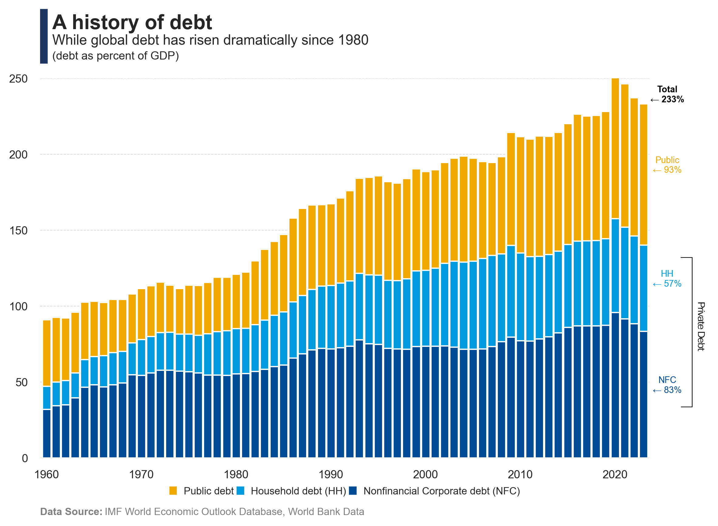
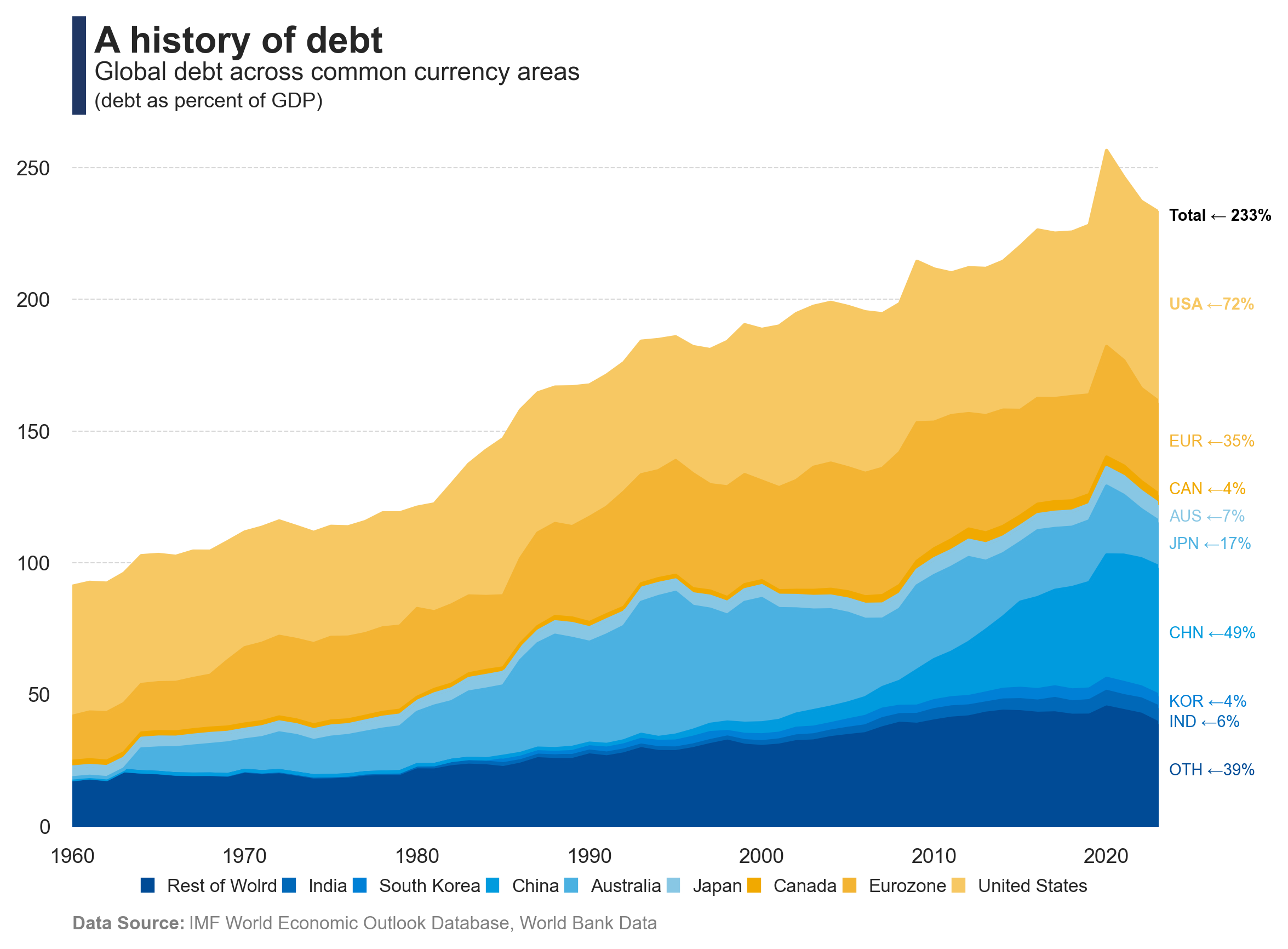
Exploring the evolution of global debt and its structure.

Published

May 18, 2026

Keywords

global debt

Summary

The chart shows the evolution of global debt over time, highlighting its structural composition. It provides insights into how debt levels have changed reached record levels during last years.

Code

# Libraries
# =====================================================================
import requests
import wbgapi as wb
import pandas as pd
import seaborn as sns
import matplotlib.pyplot as plt
import matplotlib.patches as mpatches
import matplotlib.ticker as ticker
import matplotlib.ticker as mticker
import os

# Data Extraction (Countries)
# =====================================================================
# Extract JSON and bring data to a dataframe
url = 'https://raw.githubusercontent.com/guillemmaya92/world_map/main/Dim_Country.json'
response = requests.get(url)
data = response.json()
df = pd.DataFrame(data)
df = pd.DataFrame.from_dict(data, orient='index').reset_index()
df_countries = df.rename(columns={'index': 'ISO3'})

# Data Extraction - WBD (1960-1980)
# ========================================================
# To use the built-in plotting method
indicator = ['NY.GDP.PCAP.KD', 'SP.POP.TOTL']
countries = df_countries['ISO3'].tolist()
data_range = range(1960, 1980)
data = wb.data.DataFrame(indicator, countries, data_range, numericTimeKeys=True, labels=False, columns='series').reset_index()
df_wb = data.rename(columns={
    'economy': 'ISO3',
    'time': 'Year',
    'SP.POP.TOTL': 'pop',
    'NY.GDP.PCAP.KD': 'gdpc'
})

# Filter nulls and create total
df_wb = df_wb[~df_wb['gdpc'].isna()]
df_wb['Value'] = df_wb['gdpc'] * df_wb['pop']
df_wb['Parameter'] = 'NGDPD'
df_wb = df_wb[['Parameter', 'ISO3', 'Year', 'Value']]

# Data Extraction (IMF)
# =====================================================================
#Parametro
parameters = ['NGDPD', 'PVD_LS', 'HH_LS', 'NFC_LS', 'CG_DEBT_GDP', 'GG_DEBT_GDP', 'NFPS_DEBT_GDP', 'PS_DEBT_GDP']

# Create an empty list
records = []

# Iterar sobre cada parámetro
for parameter in parameters:
    # Request URL
    url = f"https://www.imf.org/external/datamapper/api/v1/{parameter}"
    response = requests.get(url)
    data = response.json()
    values = data.get('values', {})

    # Iterate over each country and year
    for country, years in values.get(parameter, {}).items():
        for year, value in years.items():
            records.append({
                'Parameter': parameter,
                'ISO3': country,
                'Year': int(year),
                'Value': float(value)
            })
    
# Create dataframe
df_imf = pd.DataFrame(records)

# Data Manipulation
# =====================================================================
# Merge IMF and WBD
df = pd.concat([df_imf, df_wb], ignore_index=True)

# Pivot Parameter to columns and filter nulls
df = df.pivot(index=['ISO3', 'Year'], columns='Parameter', values='Value').reset_index()
df = df.dropna(subset=['PVD_LS', 'HH_LS', 'NFC_LS', 'CG_DEBT_GDP', 'GG_DEBT_GDP', 'NFPS_DEBT_GDP', 'PS_DEBT_GDP'], how='all')

# Calculate Totals
df['GDP'] = df['NGDPD']
df['Public'] = df['GG_DEBT_GDP'].fillna(df['CG_DEBT_GDP']).fillna(df['NFPS_DEBT_GDP']) * df['GDP']
df['HH'] =  df['HH_LS'] * df['GDP']
df['NFC'] = df['NFC_LS'].fillna(df['PVD_LS']) * df['GDP']

# Merge countries
df = df.merge(df_countries, how='left', left_on='ISO3', right_on='ISO3')
df = df[['ISO3', 'Country', 'Year', 'GDP', 'NFC', 'HH', 'Public']]
df = df[df['Country'].notna()]

# Groupping data
df = df.groupby('Year', as_index=False)[['GDP', 'NFC', 'HH', 'Public']].sum()

# Percent
df['NFC'] = df['NFC'] / df['GDP']
df['HH'] = df['HH'] / df['GDP']
df['Public'] = df['Public'] / df['GDP']

# Adjust table
df.drop(columns=['GDP'], inplace=True)
df = df[df['Year'] >= 1960]
df.set_index('Year', inplace=True)

print(df)

# Data Visualization
# =====================================================================
# Font and style
plt.rcParams.update({'font.family': 'sans-serif', 'font.sans-serif': ['Franklin Gothic'], 'font.size': 9})
sns.set(style="white", palette="muted")

# Palette
palette = ["#004b96", "#009bde", "#f1a900"]

# Create figure
fig, ax = plt.subplots(figsize=(8, 6))

# Crear figure and plot
df.plot(kind="bar", stacked=True, width=0.9, color=palette, legend=False, ax=ax)

# Add title and labels
fig.add_artist(plt.Line2D([0.07, 0.07], [0.87, 0.97], linewidth=6, color='#203764', solid_capstyle='butt'))
plt.text(0.02, 1.13, f'A history of debt', fontsize=16, fontweight='bold', ha='left', transform=plt.gca().transAxes)
plt.text(0.02, 1.09, f'While global debt has risen dramatically since 1980', fontsize=11, color='#262626', ha='left', transform=plt.gca().transAxes)
plt.text(0.02, 1.05, f'(debt as percent of GDP)', fontsize=9, color='#262626', ha='left', transform=plt.gca().transAxes)

# Adjust ticks and grid
plt.ylim(0, 250)
ax.yaxis.set_major_formatter(mticker.FuncFormatter(lambda x, pos: f'{int(x):,}'.replace(",", ".")))
ax.xaxis.set_major_locator(ticker.MultipleLocator(10))
plt.gca().set_xlabel('')
plt.yticks(fontsize=9, color='#282828')
plt.xticks(fontsize=9, rotation=0)
plt.grid(axis='y', linestyle='--', color='gray', linewidth=0.5, alpha=0.3)

# Custom legend values
handles = [
    mpatches.Patch(color=palette[2], label="Public debt", linewidth=2),
    mpatches.Patch(color=palette[1], label="Household debt (HH)", linewidth=2),
    mpatches.Patch(color=palette[0], label="Nonfinancial Corporate debt (NFC)", linewidth=2)
]

# Legend
plt.legend(
    handles=handles,
    loc='lower center', 
    bbox_to_anchor=(0.5, -0.12),
    ncol=4,
    fontsize=8,
    frameon=False,
    handlelength=0.5,
    handleheight=0.5,
    borderpad=0.2,
    columnspacing=0.4
)

# Add Data Source
plt.text(0, -0.15, 'Data Source:', 
    transform=plt.gca().transAxes, 
    fontsize=8,
    fontweight='bold',
    color='gray')
space = " " * 23
plt.text(0, -0.15, space + 'IMF World Economic Outlook Database, World Bank Data', 
    transform=plt.gca().transAxes, 
    fontsize=8,
    color='gray')

# Remove spines
for spine in plt.gca().spines.values():
    spine.set_visible(False)

# Add text
public = df.loc[2023, 'Public']
household = df.loc[2023, 'HH']
nonfinancial = df.loc[2023, 'NFC']

plt.text(len(df)+1.5, nonfinancial/2, f"NFC\n← {nonfinancial:.0f}%", fontsize=7, ha='center', va='bottom', color='#004b96')
plt.text(len(df)+1.5, nonfinancial + (household/2), f"HH\n← {household:.0f}%", fontsize=7, ha='center', va='bottom', color='#009bde')
plt.text(len(df)+1.5, nonfinancial + household + (public/2), f"Public\n← {public:.0f}%", fontsize=7, ha='center', va='bottom', color='#f1a900')
plt.text(len(df)+1.5, nonfinancial + household + public, f"Total\n← {nonfinancial+household+public:.0f}%", fontsize=7, ha='center', va='bottom', fontweight='bold', color='black')

# Añadir el texto estirado
plt.text(len(df)+5, (nonfinancial + household) / 2, "}", fontsize=40, ha='center', va='bottom', color='#ffffff')

# Adjust layout
plt.tight_layout()

# Save it...
download_folder = os.path.join(os.path.expanduser("~"), "Downloads")
filename = os.path.join(download_folder, f"FIG_IMF_Global_Debt.png")
plt.savefig(filename, dpi=300, bbox_inches='tight')

# Show :)
plt.show()

Code

# Libraries
# =====================================================================
import requests
import wbgapi as wb
import pandas as pd
import numpy as np
import seaborn as sns
import matplotlib.pyplot as plt
import matplotlib.patches as mpatches
import matplotlib.ticker as ticker
import matplotlib.ticker as mticker
import os

# Data Extraction (Countries)
# =====================================================================
# Extract JSON and bring data to a dataframe
url = 'https://raw.githubusercontent.com/guillemmaya92/world_map/main/Dim_Country.json'
response = requests.get(url)
data = response.json()
df = pd.DataFrame(data)
df = pd.DataFrame.from_dict(data, orient='index').reset_index()
df_countries = df.rename(columns={'index': 'ISO3'})

# Data Extraction - WBD (1960-1980)
# ========================================================
# To use the built-in plotting method
indicator = ['NY.GDP.PCAP.KD', 'SP.POP.TOTL']
countries = df_countries['ISO3'].tolist()
data_range = range(1960, 1980)
data = wb.data.DataFrame(indicator, countries, data_range, numericTimeKeys=True, labels=False, columns='series').reset_index()
df_wb = data.rename(columns={
    'economy': 'ISO3',
    'time': 'Year',
    'SP.POP.TOTL': 'pop',
    'NY.GDP.PCAP.KD': 'gdpc'
})

# Filter nulls and create total
df_wb = df_wb[~df_wb['gdpc'].isna()]
df_wb['Value'] = df_wb['gdpc'] * df_wb['pop']
df_wb['Parameter'] = 'NGDPD'
df_wb = df_wb[['Parameter', 'ISO3', 'Year', 'Value']]

# Data Extraction (IMF)
# =====================================================================
#Parametro
parameters = ['NGDPD', 'PVD_LS', 'HH_LS', 'NFC_LS', 'CG_DEBT_GDP', 'GG_DEBT_GDP', 'NFPS_DEBT_GDP', 'PS_DEBT_GDP']

# Create an empty list
records = []

# Iterar sobre cada parámetro
for parameter in parameters:
    # Request URL
    url = f"https://www.imf.org/external/datamapper/api/v1/{parameter}"
    response = requests.get(url)
    data = response.json()
    values = data.get('values', {})

    # Iterate over each country and year
    for country, years in values.get(parameter, {}).items():
        for year, value in years.items():
            records.append({
                'Parameter': parameter,
                'ISO3': country,
                'Year': int(year),
                'Value': float(value)
            })
    
# Create dataframe
df_imf = pd.DataFrame(records)

# Data Manipulation
# =====================================================================
# Merge IMF and WBD
df = pd.concat([df_imf, df_wb], ignore_index=True)

# Pivot Parameter to columns and filter nulls
df = df.pivot(index=['ISO3', 'Year'], columns='Parameter', values='Value').reset_index()
df = df.dropna(subset=['PVD_LS', 'HH_LS', 'NFC_LS', 'CG_DEBT_GDP', 'GG_DEBT_GDP', 'NFPS_DEBT_GDP', 'PS_DEBT_GDP'], how='all')

# Calculate Totals
df['GDP'] = df['NGDPD']
df['Public'] = df['GG_DEBT_GDP'].fillna(df['CG_DEBT_GDP']).fillna(df['NFPS_DEBT_GDP']) * df['GDP']
df['HH'] =  df['HH_LS'] * df['GDP']
df['NFC'] = df['NFC_LS'].fillna(df['PVD_LS']) * df['GDP']
df['Total'] = df['Public'].fillna(0) + df['HH'].fillna(0) + df['NFC'].fillna(0)

# Merge countries
df = df.merge(df_countries, how='left', left_on='ISO3', right_on='ISO3')
df = df[['ISO3', 'Cod_Currency', 'Year', 'Total', 'GDP']]
df = df[df['Cod_Currency'].notna()]
df['Region'] = np.where(df['Cod_Currency'] == 'EUR', 'EUR', np.where(df['ISO3'].isin(['USA', 'CHN', 'JPN', 'AUS', 'IND', 'KOR', 'CAN']), df['ISO3'], 'OTH'))

# Groupping data
df = df.groupby(['Year', 'Region'], as_index=False)[['GDP', 'Total']].sum()

# Percent
df['Total'] = df['Total'] / df.groupby('Year')['GDP'].transform('sum')

# Adjust table
df.drop(columns=['GDP'], inplace=True)
df = df[df['Year'] >= 1960]
df = df.pivot_table(index='Year', columns='Region', values='Total', aggfunc='sum', fill_value=0)
df = df[['OTH', 'AUS', 'CAN', 'CHN', 'IND', 'JPN', 'KOR', 'EUR', 'USA']]

print(df)

# Data Visualization
# =====================================================================
# Font and style
plt.rcParams.update({'font.family': 'sans-serif', 'font.sans-serif': ['Franklin Gothic'], 'font.size': 9})
sns.set(style="white", palette="muted")

df = df[['OTH', 'IND', 'KOR', 'CHN', 'JPN', 'CAN', 'AUS', 'EUR', 'USA']]

# Palette
palette = [
    "#004b96",  # OTH
    "#0068b8",  # IND
    "#0080d6",  # KOR
    "#009bde",  # CHN
    "#4bb1e1",  # JPN
    "#88c7e4",  # CAN
    "#f1a900",  # AUS
    "#f3b433",  # EUR
    "#f7c863"   # USA
]

# Create figure
fig, ax = plt.subplots(figsize=(8, 6))

# Crear figure and plot
df.plot(kind="area", stacked=True, color=palette, legend=False, ax=ax)

# Add title and labels
fig.add_artist(plt.Line2D([0.07, 0.07], [0.87, 0.97], linewidth=6, color='#203764', solid_capstyle='butt'))
plt.text(0.02, 1.13, f'A history of debt', fontsize=16, fontweight='bold', ha='left', transform=plt.gca().transAxes)
plt.text(0.02, 1.09, f'Global debt across common currency areas', fontsize=11, color='#262626', ha='left', transform=plt.gca().transAxes)
plt.text(0.02, 1.05, f'(debt as percent of GDP)', fontsize=9, color='#262626', ha='left', transform=plt.gca().transAxes)

# Adjust ticks and grid
plt.ylim(0, 260)
plt.xlim(1960, 2023)
ax.yaxis.set_major_formatter(mticker.FuncFormatter(lambda x, pos: f'{int(x):,}'.replace(",", ".")))
ax.xaxis.set_major_locator(ticker.MultipleLocator(10))
plt.gca().set_xlabel('')
plt.yticks(fontsize=9, color='#282828')
plt.xticks(fontsize=9, rotation=0)
plt.grid(axis='y', linestyle='--', color='gray', linewidth=0.5, alpha=0.3)

# Custom legend values
handles = [
    mpatches.Patch(color=palette[0], label="Rest of Wolrd", linewidth=2),
    mpatches.Patch(color=palette[1], label="India", linewidth=2),
    mpatches.Patch(color=palette[2], label="South Korea", linewidth=2),
    mpatches.Patch(color=palette[3], label="China", linewidth=2),
    mpatches.Patch(color=palette[4], label="Australia", linewidth=2),
    mpatches.Patch(color=palette[5], label="Japan", linewidth=2),
    mpatches.Patch(color=palette[6], label="Canada", linewidth=2),
    mpatches.Patch(color=palette[7], label="Eurozone", linewidth=2),
    mpatches.Patch(color=palette[8], label="United States", linewidth=2)
]

# Legend
plt.legend(
    handles=handles,
    loc='lower center', 
    bbox_to_anchor=(0.5, -0.12),
    ncol=9,
    fontsize=8,
    frameon=False,
    handlelength=0.5,
    handleheight=0.5,
    borderpad=0.2,
    columnspacing=0.4
)

df = df[['OTH', 'IND', 'KOR', 'CHN', 'JPN', 'AUS', 'CAN', 'EUR', 'USA']]

# Add text
oth = df.loc[2023, 'OTH']
ind = df.loc[2023, 'IND']
kor = df.loc[2023, 'KOR']
chn = df.loc[2023, 'CHN']
jpn = df.loc[2023, 'JPN']
can = df.loc[2023, 'AUS']
aus = df.loc[2023, 'CAN']
eur = df.loc[2023, 'EUR']
usd = df.loc[2023, 'USA']

plt.text(1.01, 0.07, f"OTH ←{oth:.0f}%", fontsize=7, ha='left', va='bottom', color=palette[0], transform=plt.gca().transAxes)
plt.text(1.01, 0.14, f"IND ←{ind:.0f}%", fontsize=7, ha='left', va='bottom', color=palette[1], transform=plt.gca().transAxes)
plt.text(1.01, 0.17, f"KOR ←{kor:.0f}%", fontsize=7, ha='left', va='bottom', color=palette[2], transform=plt.gca().transAxes)
plt.text(1.01, 0.27, f"CHN ←{chn:.0f}%", fontsize=7, ha='left', va='bottom', color=palette[3], transform=plt.gca().transAxes)
plt.text(1.01, 0.4, f"JPN ←{jpn:.0f}%", fontsize=7, ha='left', va='bottom', color=palette[4], transform=plt.gca().transAxes)
plt.text(1.01, 0.44, f"AUS ←{aus:.0f}%", fontsize=7, ha='left', va='bottom', color=palette[5], transform=plt.gca().transAxes)
plt.text(1.01, 0.48, f"CAN ←{can:.0f}%", fontsize=7, ha='left', va='bottom', color=palette[6], transform=plt.gca().transAxes)
plt.text(1.01, 0.55, f"EUR ←{eur:.0f}%", fontsize=7, ha='left', va='bottom', color=palette[7], transform=plt.gca().transAxes)
plt.text(1.01, 0.75, f"USA ←{usd:.0f}%", fontsize=7, ha='left', va='bottom', fontweight='bold', color=palette[8], transform=plt.gca().transAxes)
plt.text(1.01, 0.88, f"Total ← {oth+ind+kor+chn+jpn+can+aus+eur+usd:.0f}%", fontsize=7, ha='left', va='bottom', fontweight='bold', color='black', transform=plt.gca().transAxes)

# Add Data Source
plt.text(0, -0.15, 'Data Source:', 
    transform=plt.gca().transAxes, 
    fontsize=8,
    fontweight='bold',
    color='gray')
space = " " * 23
plt.text(0, -0.15, space + 'IMF World Economic Outlook Database, World Bank Data', 
    transform=plt.gca().transAxes, 
    fontsize=8,
    color='gray')

# Remove spines
for spine in plt.gca().spines.values():
    spine.set_visible(False)

# Adjust layout
plt.tight_layout()

# Save it...
download_folder = os.path.join(os.path.expanduser("~"), "Downloads")
filename = os.path.join(download_folder, f"FIG_IMF_Global_Debt_Countries.png")
plt.savefig(filename, dpi=300, bbox_inches='tight')

# Show it :)
plt.show()